Hobby Projects
Modelling MRI Pulses
Nuclear magnetic resonance
In Magnetic Resonance Imaging (MRI) the nuclear spins in our body are placed in a strong homogeneous magnetic field $\mathsf{B_0}$ excited into a rotational state by radio frequency (RF) pulse. Once excited by an RF pulse, the nuclear spins rotate in phase, producing a measurable macroscopic magnetisation $\mathsf{ M(t)}$, which decays over time according to tissue-specific time scales called $\mathsf{T_1}$ and $\mathsf{T_2}$. This measurable signal is known in MRI as “free induction decay” (FID). The shape of the RF pulse is crucial in determining the frequency range to be excited. In MRI, the ability to excite only a specific, narrow frequency range is crucial. In fact, this is necessary in order to obtain spatial information, which can finally result in medically useful images.
However, the relationship between the shape of the pulse and the corresponding frequency response is far from trivial. It can be modeled mathematically by the so-called Bloch Equations:
$$\mathsf{\frac{d M_x(t)}{dt} = -\Delta\omega M_y(t) - \gamma B_{1,y}(t)M_z(t) - \frac{M_x(t)}{T_2} }$$ $$\mathsf{\frac{d M_y(t)}{dt} = \Delta\omega M_x(t) + \gamma B_{1,x}(t)M_z(t) - \frac{M_y(t)}{T_2} }$$ $$\mathsf{\frac{d M_z(t)}{dt} = \gamma B_{1,y}(t)M_x(t) - \gamma B_{1,x}(t)M_y(t) - \frac{M_z(t) - M_z^0}{T_1} }.$$
Here, $\gamma$ is a physical constant known as the gyromagnetic ratio and $\mathsf{B_1}$ is the magnetic field corresponding to the applied RF pulse. Moreover, $\mathsf{\Delta\omega}$ denotes the deviation in frequency from the Larmor frequency of the tissue. Ideally, a RF pulse should be able to excite $\mathsf{M_x}$, $\mathsf{M_y}$, $\mathsf{M_z}$ only in a narrow band around $\mathsf{\Delta\omega=0}$.
Numerical modelling
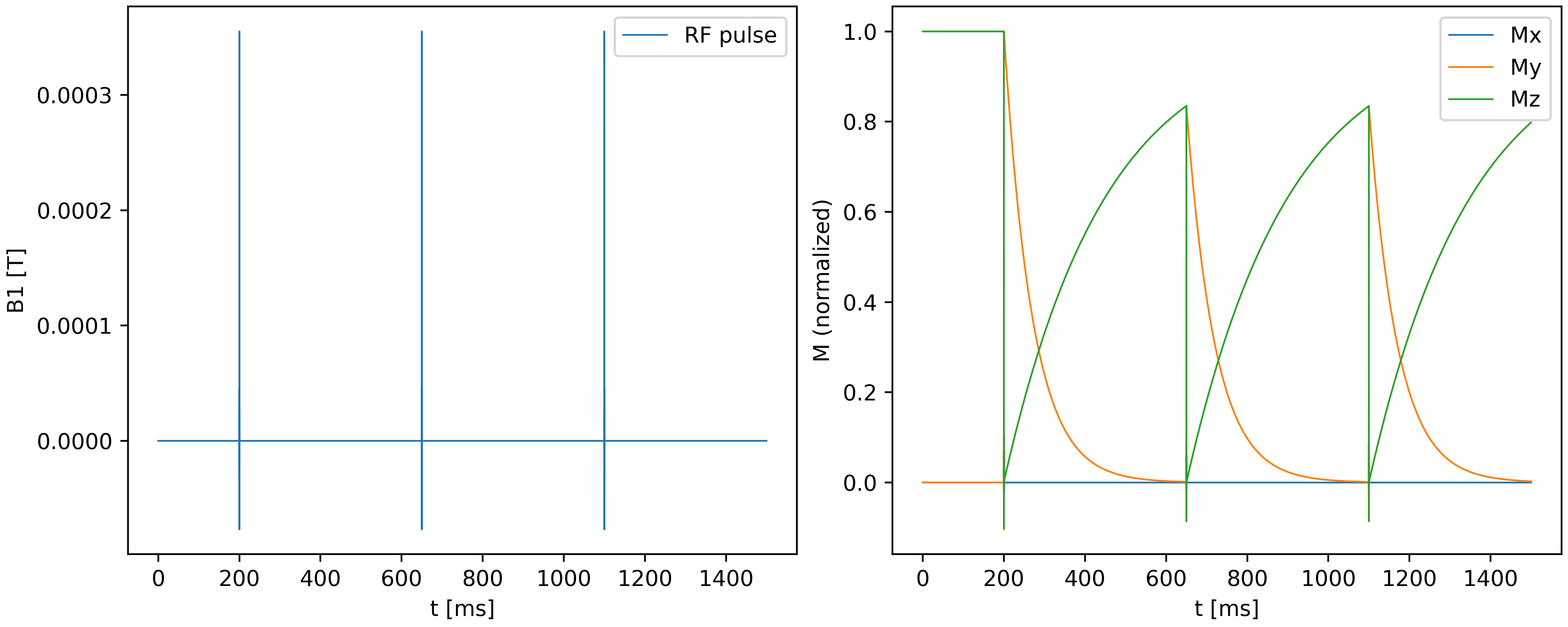
I have written a numerical solver for the Bloch equations in Python, which allows to understand both qualitative and quantitative features of MR pulse sequences. The code is open source and available on github.com/frank-roesler/bloch_solver. The following figure illustrates the on-resonance effect ($\mathsf{\Delta\omega=0}$) of a sinc shaped RF pulse on the magnetisation $\mathsf M$. The component $\mathsf{M_y}$ gets excited after each of the pulses, after which it decays exponentially. Observe how the first pulse achieves maximal excitation (i.e. $\mathsf{M_y}=1$), while all subsequent pulses only achieve partial excitation (right hand plot), due to incomplete $\mathsf T_1$ recovery. This is exactly what is expected theoretically and observed experimentally (see here, for example).

Spin echo and field gradients
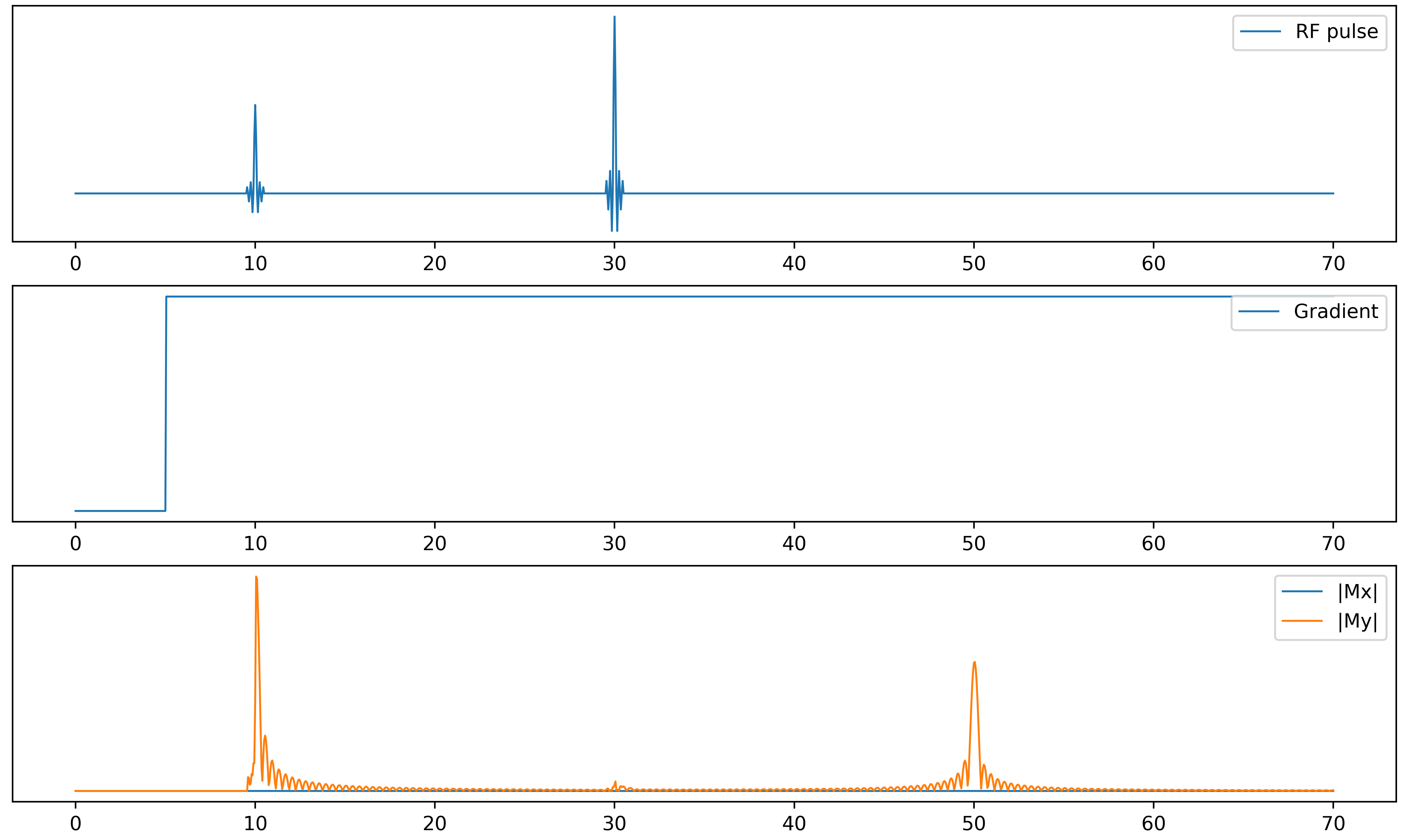
The code can be used to explore more qualitative features of MRI pulse sequences. Most modern imaging sequences exploit an effect known as “spin echo”. This effect allows to partially reverse the $\mathsf{T_2}$ decay through clever usage of RF pulses and magnetic field gradients. The idea is to re-align nuclear spins that have gotten out of phase due to magnetic field inhomogeneities. This can either be achieved via a so-called 180º RF pulse, or through two opposite magnetic field gradients. The following figure illustrates the former case. An initial pulse excites the magnetisation, after which it decays due to field inhomogeneities (modeled here by a constant gradient, for simplicity). After a time $\mathsf{T_E/2}$ another pulse (the 180º pulse) is applied. The numerics shows another peak appearing seemingly out of nowhere at time $\mathsf{T_E}$ after initial excitation. This is known in MRI as “spin echo”.

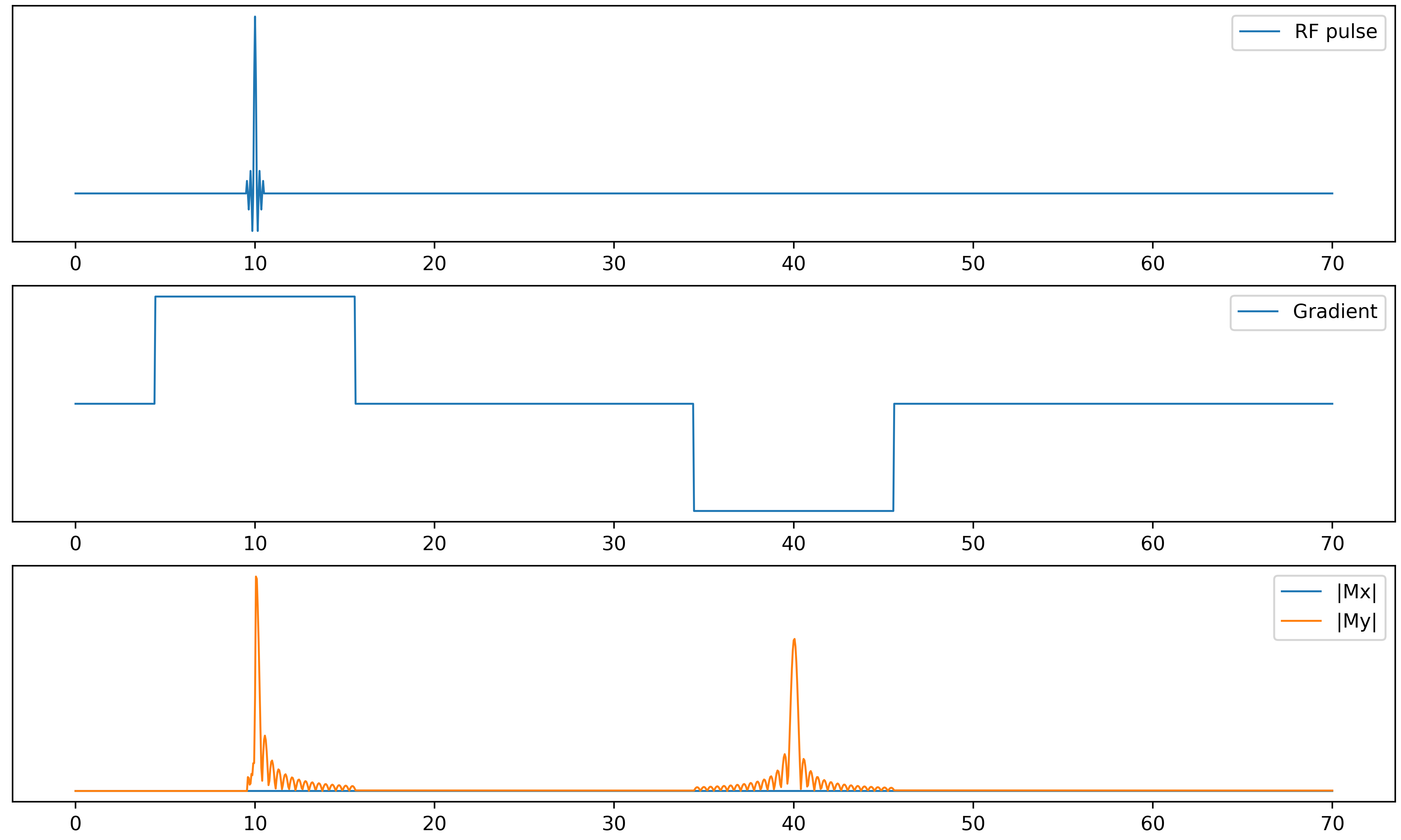
The latter case, known as “gradient echo”, is illustrated in the next figure. Here, rather than a second RF pulse, a magnetic field gradient is applied in two opposite directions. The initial gradient causes dephasing of the spins, leading to rapid signal decay, while the second gradient achieves a rephasing, which recovers the original signal.

All these effects can be observed experimentally using actual MRI scanners. The Bloch equations and some basic numerics allow us to understand and predict them and all we need is a personal Laptop!